If you have collected a data sample and wish to compute descriptive statistics for it, this is the place. For a given sample, we compute the mean, standard deviation, variance, skewness, kurtosis, quartiles, median, min, max. Additionally, we provide a statistic that detects deviation from normality due to either skewness or kurtosis based on D'Agostino's K-squared test.

Just paste your sample data in the text box and press "Calculate". (numbers separated by at least one space)

Brief summary - Descriptive Statistics

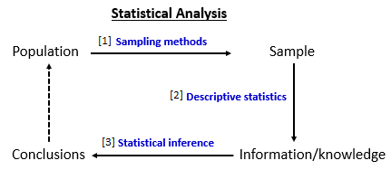
Descriptive statistics is the initial step of the analysis one can make from your data sample. It is used to describe and summarize the data.  It can be situated in the context of Statistical Analysis where the first step is the data collection through the use of Sampling methods. The second step is the Descriptive Statistics itself, summarizing the knowledge we can get from the sample and showing important characteristics that describes it. And finally, another step is the Statistical inference that is able to infer properties of a population, for example by testing hypotheses and deriving estimates.

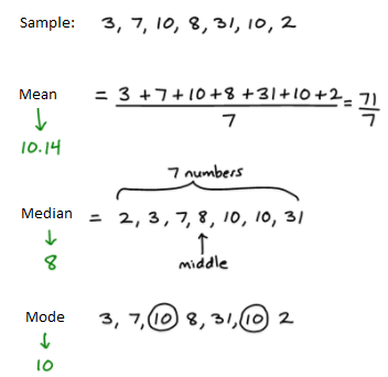
In terms of Descriptive Statistics, important statistics (measures or characteristics) are measures of central tendency and measures of variability or dispersion. Measures of central tendency include the  mean, median and mode, while measures of variability include the standard deviation, variance, quartiles, kurtosis and skewness, the minimum and maximum values of the variables and others.

Measures of central tendency are so named because they indicate a point around which the data are concentrated. This point tends to be the center of data distribution.

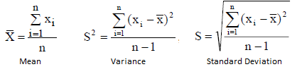
The arithmetic mean or simply the mean or average is the sum of a collection of numbers divided by the number of numbers in the collection (sample). Under a geometric view, the mean of a distribution is the center of gravity, it represents the break-even point of a set of data. It is the central tendency measure most used to represent the mass of data.

The Mode is the value that occurs most often, or the value that corresponds to the class interval with the highest frequency. Mode, differently from the mean, is not affected by extreme values.

The Median is an alternative measure to the arithmetic mean to represent the center of the distribution. The median of a set of measures (x1, x2, x3, ..., xn) is a value M such that at least 50% of the measurements are less than or equal to M and at least 50% of the measurements are greater than or equal to M. In other words, 50% of the measurements are below the median and 50% higher. If the number of values is even, it can be calculated as the mean of the two middle values. Median, like the mode, is not affected by extreme values.

In terms of measure of variability (statistical dispersion), common measures are: interquartile range, standard deviation, variance, skewness, kurtosis, range (total amplitude).

Another measure is the Quartile. The first quartile is defined as the middle number between the smallest number and the median of the data set. The second quartile is the median of the data. The third quartile is the middle value between the median and the highest value of the data set. The Interquartile range IQR is the first quartile subtracted from the third quartile reason it is also called midspreadmiddle 50%.

Variance can be calculated as the average of the square of deviations from the mean. A deviation is the difference between each observed value and the mean.

The Standard deviation is the square root of the variance.

The Range is the interval from the minimum value to the maximum value of the sample.

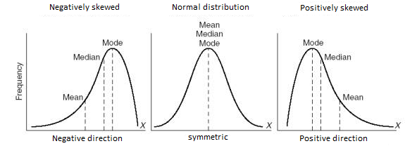
Skewness and Kurtosis are considered Measures of Shape and give information about the shape of the distribution.

In terms of skewness, if the bulk of the data is at the left and the right tail is longer, we say that the distribution is skewed right or positively skewed; if the peak is toward the right and the left tail is longer, we say that the distribution is skewed left or negatively skewed. A normal distribution has a skewness of zero.

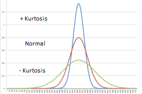
In terms of kurtosis, the question is about the central peak: is it high and sharp, or short and broad? The height and sharpness of the peak relative to the rest of the data are measured by a number called kurtosis. Higher values indicate a higher, sharper peak; lower values indicate a lower, less distinct peak. A normal distribution has a kurtosis of 3. The is the reason the term excess kurtosis is the kurtosis minus 3. 

There are many ways to assess normality. One test is the D'Agostino-Pearson omnibus test, so called because it uses the test statistics for both skewness and kurtosis to come up with a single p-value. For 95% confidence level, if p-value is smaller than 0.05 you can assume the distribution is not normal. Better results for sample sizes above 20.