Introduction    Here we provide examples about how the Universal Probability Calculator (UPC) can be used to calculate probalities for normal and non-normal data. We also perform the calculations using Microsoft Excel and Minitab, so the user can learn how to compute probabilities in such tools and the difference when compared with UPC.       Going straight to the point, when using UPC you do not need to be worried if the distribution is normal or not, you just need to paste your data and press "calculate". When using other tools, you need to do this analysis at first in order to decide about the next steps, which is complex and full of tricks that can mislead the user to make bad decisions.  Example 1 (normal distribution) Description of the problem: Assume you measured the commuting time from your house to the office 15 times. By doing that you realize that the average time is 53 minutes. You also wish to know the odds of taking up to 1 hour to go to the office. Measured values (minutes) 52.7 43.5 43.3 59.2 47.8 65.2 38.7 51.7 53.6 54.3 67.9 49.7 51.6 63.8 53.6 Solution using the “Universal Probability Calculator (UPC)”: The first step is showed in the following figure: In the second step, copy and paste the values directly to the field: After clicking on the button “Calculate” a message is displayed saying that the odds are 81.9%. Solution using “Excel - Windows”: On the Excel menu, Data -> Data Analysis -> Descriptive Statistics to get table below: Mean 53.10165 Standard Error 2.137853 Median 52.6883 Mode #N/A Standard Deviation 8.279871 Sample Variance 68.55626 Kurtosis -0.36244 Skewness 0.208165 Range 29.1862 Minimum 38.7058 Maximum 67.892 Sum 796.5247 Count 15 Because Kurtosis and Skewness are close to zero, we can assume that the distribution is normal, or at least close to it. The sample size is 15 which is small. We also do not know the variance of the population. For all these reasons it is appropriate to use a Student distribution. 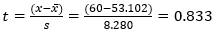With degree of freedom of 14, we have:        Using Excel command T.DIST(0.833,14,1), we get that the probability of having a value up to 60 minutes is 79.06%. 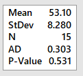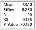Solution using “Minitab”: Initially we perform a test of goodness for a normal distribution. On Minitab: Stat-> Basic Statistics -> Normality Test. For Anderson-Darling and Kolmogorov-Smirnov we have the results on the right, both not rejecting the null hypothesis of normality. Therefore, it is plausible to assume the distribution is normal.     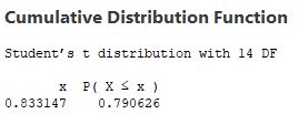Because sample size is small and we do not know the variance of the population, we use Student distribution. On Minitab: Calc -> Probability Distributions-> t . Select “cumulative probability”, and in the field “input constant” entry 0.833  (same value previously used for the Excel solution). By doing so, we get the answer (on the right) saying the probability of having a value smaller than 60 minutes is 79.06%. Discussion of the results Initially, regarding the source of the data, it was generated a population of 20000 values using the software Matlab, function: (randn(20000,1) * 5 ) + 50. From this population, we collect 15 values by chance (our working sample). Summary of the results: UPC-Dunamath Excel Minitab Correct answer 81.9% 79.06% 79.06% 97.72%   Excel and Minitab returned the same result because they both used Student Distribution with the same parameter t. Both assumed normal distribution which is correct in this case because the population was generated from a normal distribution. However, the mean and standard deviation parameters used to calculate t  are significantly wrong. For the sample, mean and standard deviation are 53.1 and 8.28 respectively, while for the population they are 50 and 5. It explains the big error of the answer. Other point is that even using Excel and/or Minitab correctly, it is likely that the decision maker will believe in the result (79.06%) and make his decision. These tools do not give information about the accuracy of the answer and many times the users are not even aware of the existence of uncertainty in the result. The Universal Probability Calculator (UPC) retuned a probability of 81.9%, a little bit better than the others, and it also reports a small confidence level of 64%, alerting the user about it. The UPC not only computes the probability in very simple and straight way, but also gives an estimate of the uncertainty present in the result. By doing so, it seems to be fairer with the decision maker. If he wishes to have a smaller uncertainty, he needs to increase the size of the sample. Note that we are not calculating the probability of having a sample mean smaller than 1 hour. That would be a different question. Example 2 (non-normal distribution) Problem description: A product engineer is studying the life time of a hard drive disc. In one experiment it is measured the life time in hours of 10 discs. Results in the following table: 1988.77 2026.69 2074.94 2018.67 1973.65 1921.29 1941.77 1937.22 1895.03 1942.83   A)     What is the probability of having a disc lasting longer than 1900 hours? Solution using the “Universal Provability Calculator (UPC)”: Step 1 as follows: Note that you could have selected  the symbol >=, but because the date refers to consitnuous variables, that is not relevant. Step 2 as follows, copying and pasting the data: After clicking on “Calculate” is displayed a message saying that the probability of having a disc lasting longer than 1900 hours is 90.56%. Solution using “Excel - Windows”: Excel Menu: Data -> Data Analysis -> Descriptive Statistics to get the following table: Mean 1972.086 Standard Error 17.48647 Median 1958.24 Mode #N/A Standard Deviation 55.29706 Sample Variance 3057.765 Kurtosis -0.35796 Skewness 0.552605 Range 179.91 Minimum 1895.03 Maximum 2074.94 Sum 19720.86 Count 10 Because Kurtosis and Skewness are close to zero, it is plausible to assume the distribution is normal or approximately normal. The sample size is small and we do not know the variance of the population, therefore we decide to use Student distribution. 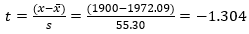With degree of freedom 9, we have: Using the Excel command T.DIST(-1.304,9,1), we have that the probability of having a value greater than 1900 is 88.8%. Solution using “Minitab”: Initially we perform a test of goodness for a normal distribution. On Minitab: Stat-> Basic Statistics -> Normality Test. For Anderson-Darling and Kolmogorov-Smirnov we have the results on the right, both not rejecting the null hypothesis of normality. Therefore, it is plausible to assume the distribution is normal.   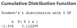Because sample size is small and we do not know the variance of the population, we use Student distribution. On Minitab: Calc -> Probability Distributions-> t. Select “cumulative probability”, and in the field “input constant” entry -1.304 (same t computed in Excel). The answer is on the right, where the probability is (100-11.2)=88.8%. B)      Regarding the probability you have just calculated, how sure you are? Using UPC-Dunamath, a message is displayed saying: “We are 68% confidence that the true value is between 85.56% and 95.56%”. It means, we are 68% confident the true value falls within this interval. It also means that if you collect more 15 samples to repeat the test, and keep doing that many times, at least 68% of the probabilities will fall within the interval. Note that we do not have this information from Excel or Minitab. C)      In order to improve the confidence level, you get the lifetime of others 30 discs, and you repeat the test using also the previous sample, totalling a sample of 40 discs. What is the probability of having a disc lasting longer than 1900 hours? 1988.77 2026.69 2053.48 2140.11 2132.87 2062.56 1970.53 2164.22 2074.94 2018.67 1982.92 1924.92 2154.11 1788.89 2046.63 2019.41 1973.65 1921.29 1968.29 1753.65 1972.47 2028.2 2000.97 1960.72 1941.77 1937.22 1943.67 1957.47 1909.35 2018.27 2102.17 1695.47 1895.03 1942.83 2063.94 1678.59 1948.96 2050.25 1899.61 2058.53 Solution using the “Universal Provability Calculator (UPC)”: Step 1: Step 2 (copy and paste data): Note there are more values on the right of the field in the picture. After clicking on “Calculate” is displayed a message saying that the probability of having a disc lasting longer than 1900 hours is 85.09%, with 79% confidence that the true value is between 80.09% and 90.09%. Solution using “Excel - Windows”: Excel menu: Data -> Data Analysis -> Descriptive Statistics: Mean 1979.302 Standard Error 17.43848 Median 1978.285 Mode #N/A Standard Deviation 110.2906 Sample Variance 12164.02 Kurtosis 1.321178 Skewness -0.90893 Range 485.63 Minimum 1678.59 Maximum 2164.22 Sum 79172.09 Count 40 Kurtosis and Skewness are NOT close to zero, not too far too, but in this case, it is safer not assume the distribution is normal. In Excel there is no straight method to deal with non-normal data. One alternative is to assume the data is not far from normal, and use Student Distribution, with t = (1900-1979.30)/110.29 = -0.719,  Excel command T.DIST(-0.719,39,1), resulting in 76.2%.  Another alternative is to use an Empirical Distribution Function (EDF), as showed in the next step.   A table with the Empirical Distribution is showed as follows: X(i) q < X(i) EDF <x EDF > x 1678.59 1 0.025 0.975 1695.47 2 0.05 0.95 1753.65 3 0.075 0.925 1788.89 4 0.1 0.9 1895.03 5 0.125 0.875 1899.61 6 0.15 0.85 1909.35 7 0.175 0.825 1921.29 8 0.2 0.8 1924.92 9 0.225 0.775 1937.22 10 0.25 0.75 1941.77 11 0.275 0.725 1942.83 12 0.3 0.7 1943.67 13 0.325 0.675 1948.96 14 0.35 0.65 1957.47 15 0.375 0.625 1960.72 16 0.4 0.6 1968.29 17 0.425 0.575 1970.53 18 0.45 0.55 1972.47 19 0.475 0.525 1973.65 20 0.5 0.5 X(i) q < X(i) EDF <x EDF > x 1982.92 21 0.525 0.475 1988.77 22 0.55 0.45 2000.97 23 0.575 0.425 2018.27 24 0.6 0.4 2018.67 25 0.625 0.375 2019.41 26 0.65 0.35 2026.69 27 0.675 0.325 2028.2 28 0.7 0.3 2046.63 29 0.725 0.275 2050.25 30 0.75 0.25 2053.48 31 0.775 0.225 2058.53 32 0.8 0.2 2062.56 33 0.825 0.175 2063.94 34 0.85 0.15 2074.94 35 0.875 0.125 2102.17 36 0.9 0.1 2132.87 37 0.925 0.075 2140.11 38 0.95 0.05 2154.11 39 0.975 0.025 2164.22 40 1 0   In the Empricial Distributon table, in the first column we have the data sorted in ascending order. In the second column we have for each value the amount of values smaller or equal to the current value (which coincides with the row number). In the third column we have the value of the second column divided by the sample size resulting in a cumulative frequency. Finally, in the fourth column we have the complement of the third column. We want to calculate the probability of having a value greater than 1900. In the table, the value 1900 is between lines 6 and 7 (1899.61 and 1909.35). By doing so it is possible to say that the probability is around 82.5% and 85%. Note that there is no guarantee the true value is within this interval. But for a non-normal data, this is a simple method to give a notion of the probability. Solution using “Minitab”: Initially we perform a test of goodness for a normal distribution. On Minitab: Stat-> Basic Statistics -> Normality Test. For Anderson-Darling the null hypothesis of normality is rejected. Therefore, it is not plausible to assume the distribution is normal. 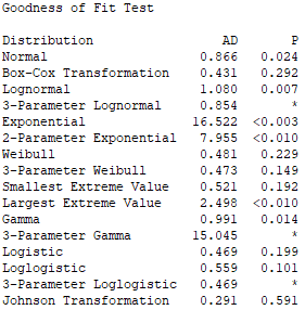Because the distribution is not normal, we need to estimate the type of the distribution. Minitab menu:  Stat > Quality Tools > Individual Distribution Identification. We get the table on the right, with an Anderson Darling test applied to different types of distribution. In general, all distributions with P smaller than 0.05 are immediately discarded. From the remaining ones, we get the one with greatest P value. In our case, the first is “Johnson Transformation”, then “Box-Cox Transformation”, and after that, “Weibull”. Because the first two are transformations and not native distributions, and also, there is no straight method to use them in Minitab, we pick the “Weibull” distribution. With the previous table we also have the following table with the parameter of each distribution. In our case, for “Weibull”, there are 2 parameters: 22.30053 (shape) and 2027 (scale). In the next step, on Minitab menu: Calc -> Probability Distributions->Weibull. Select “cumulative probability”, type the 2 values of the parameters, in the field “input constant”, type the value 1900.  By doing so, we have the answer as follows:                         We want the probability of having values greater than 1900, so we have (1-0.2098) = 0.7902 = 79.02%.             Phew!!! Finally! Discussion of the results: Initially, regarding the source of the data, we generated 20000 values using the software Matlab, function: wblrnd(2042.6,25.8773,20000,1)  generating a population with Weibull distribution, mean 2000.3 and standard deviation 97.192. From that, we collect our samples by chance.                        For the first sample (N=10): UPC-Dunamath Excel Minitab Correct answer 90.56% 88.8% 88.8% 85.82%  For the extended sample (N=40): UPC-Dunamath Excel (using Student Distribution) Excel (empirical distribution) Minitab Correct answer 85.09% 76.2% [82.5% - 85%] 79.02% 85.82%   In the first table (N=10), we see that Excel and Minitab returned the same result because they both used Student distribution with the same t . But note that, despite the approval in the test of goodness for normal distribution, the correct distribution is Weibull. The mean and standard deviation of the sample are 1972.09 and 55.30 respectively, while for the population we have 2000.3 and 97.192. Note that despite the fact we have assumed the wrong distribution the probability error is small, which might be just lucky, for example a numerical coincidence influenced by the relation between mean and standard deviation. For UPC, the probability is 90.56%, with 68% confidence that the true value is between 85.56% and 95.56%. The confidence is low due to the small sample which is an alert for the user, not provided by the other tools. Despite that, the true value is within the interval. In the second table (N=40), both in Excel and Minitab we rejected the assumption of normality. For Excel, we proposed the utilization of the Empirical Distribution Function just to have an idea of the probability, obtaining a value around 82.5% and 85%, which compared with the correct answer is a plausible value. Using Minitab, after a hard work identifying a suitable distribution type, its parameters, and performing the calculation, the result was even worse than the case with N=10. This is an inconvenient but possible, because we are using small samples, and maybe the additional samples are less representative of the population than the initial sample, or it is just a numerical coincidence. For UPC, the probability is 85.09%, with 79% confidence that the true value is between 80.09% and 90.09%. Compared with N=10, the confidence level increased significantly due to a bigger sample size. The error is smaller than Excel and Minitab, and the true value is with the estimated interval. By this example, we see how complicated these analyses can become. It is complicated to calculate a value for the probability, and after that, you still do not know the uncertainty of the result. The Universal Probability Calculator (UPC) makes this calculation much easier, and also gives an estimate for the uncertainty involved. You do not need to be worried with all statistical assumptions and trick details, it is everything treated by our algorithm.